Difficulty of training RNNs
A concise summary of the paper titled “On the difficulty of training Recurrent Neural Networks” by Bengio…
What to do ?
For exploding gradients : Clip the gradient norm to something easy to process For vanishing gradients : Use a soft constraint to discourage this case
Reccurent Neural Networks are similar to vanilla multilayer perception networks, with connections among hidden units associated with a time delay. This enables the model to retain past inputs and understand temporal connections between inputs at different time instances. Powerful and simple, these are hard to train due to instable gradient operations (read about Vanishing and Exploding Gradients)
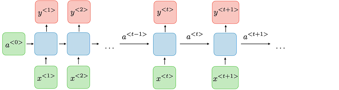
A cost function (ε) measures the performance of the function on some given tasks and it can be broken down into individual $ costs ~for ~each ~step (t), ~ ε = \sigma ε_t $ ; where ε_t is the loss/cost at timestamp t.
To calculate the gradients, we make use of BackPropogation Through Time (BPTT), for which the recurrent architecture is unrolled and the gradients flow ‘backwards’ through time.
Why is training hard ?
A large increase in the norm of the gradient can be caused by exponential growth in the long-term components; which is called exploding gradients. Conversely, vanishing gradients are when the long-term components move exponentially towards 0 norm, making it impossible for the model to learn / understand relations between incidents / words that are far apart (temporally distant events).
For gradients to explode, the largest eigenvalue (λ) of the weight matrix should be larger than 1, and for long-term components to be lost (gradients are lost) λ < 1 is sufficient.
State Space & Attraction Basins
For any dynamic system, the parameter converges due to the repeated application / effect of several possible attractor states (imagine them as magnets). These attractors define model behavior and the state space (all possible values that the parameter can take) is divided into multiple basins of attraction. If a model is initialized in one basin, convergence is likely to be observed in the same basin.
As per basic Dynamic Systems Theory, the parameter value changes slowly almost everywhere except for Bifurcation Boundaries, where large change occurs. Crossing these boundaries can cause gradients to explode, as a small update in the parameter value results in it switching over to another basin, which a different attractor created.
Fun Fact : If the error-gradients fall to zero, it means the output does not depend on the particular cell / all cells before the current cell. This also means that the model is close to convergence for some attractor at state k.
Geometric Interpretation
When the 1ˢᵗ derivative explodes, so does the 2ⁿᵈ order derivative, generally along some direction leading to a wall-like surface in the error space.

Parameters are initialized with small values thus limiting the spectral radius of $W_{rec}$ (weights of the recurrent network) to less than 1, limiting the chances of Exploding Gradients. This limits the model to a single regime / attractor, where any information inserted dies out exponentially fast in time.
Another Fun fact : In high dimensional spaces, long term components are often orthogonal to short term components.
Exploding gradients are linked with tasks that require long memory traces, as initially, the model operates in a one-attractor regime. More memory translates to a larger spectral radius and when this value crosses a certain threshold the model enters rich regimes (under the influence of multiple attractors) where gradients are much more likely to explode.
What can we even do ?
A simple way to deal with sudden increases in gradient norms is to rescale them whenever the norm breaches a threshold. Simple to implement and computationally cheap, this introduces an additional hyperparameter, the threshold.
To deal with vanishing gradients we can make use of a regularization term that forces the error signal to not vanish as it travels back in time while BPTT. The regularizer forces the model to preserve the norm in only relevant directions.
What next ?
- A paper summary of “Understanding LSTM” by Morris and Staudemeyer
- A paper summary of “xLSTM : Extended LSTMs”
- Implementation of sLSTM and mLSTM blocks